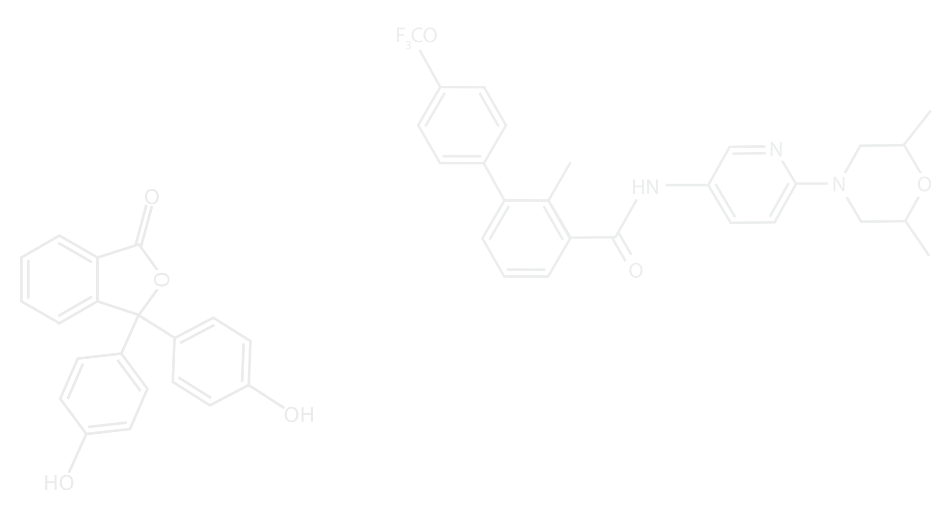
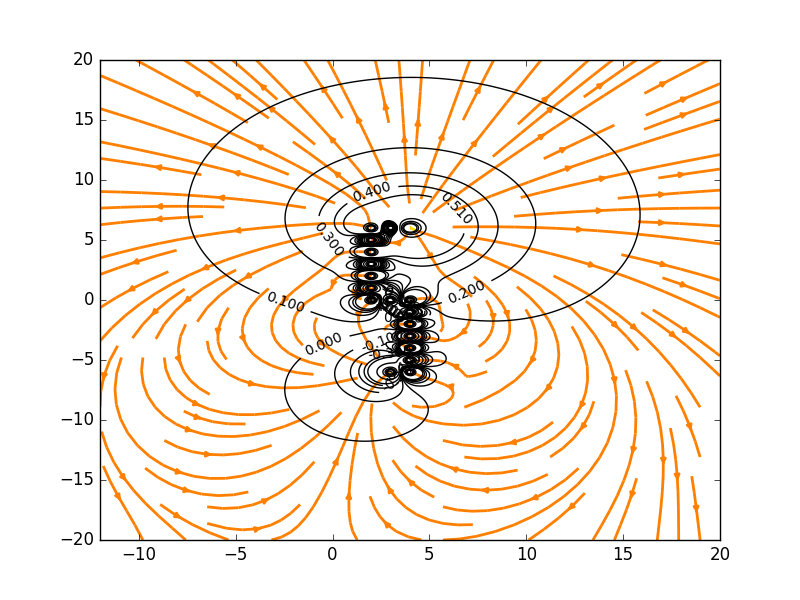
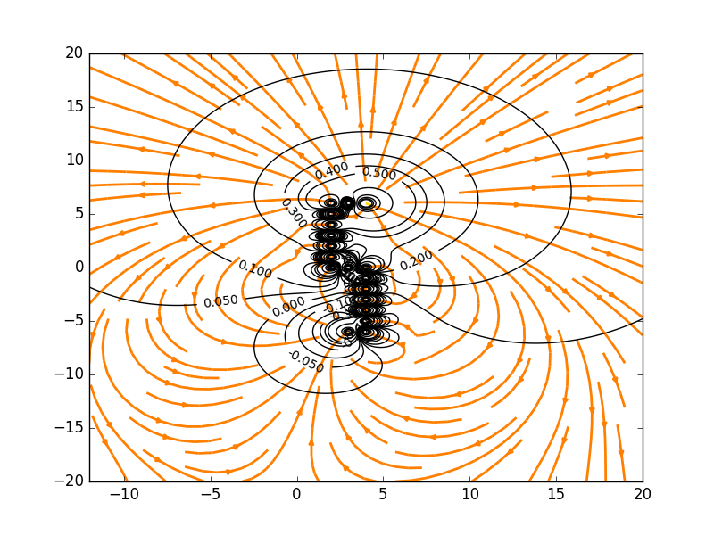
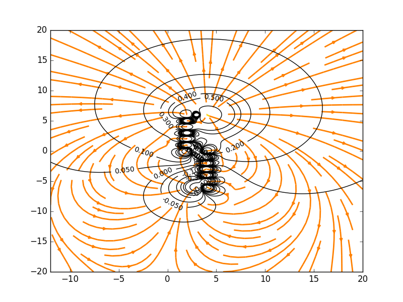
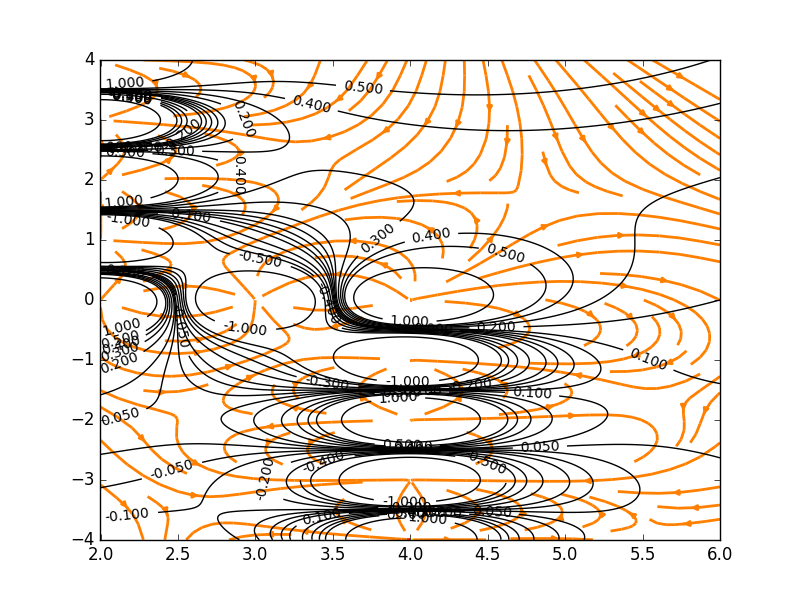
Electric Field Lines and Equipotential Surfaces with Charges Spelling "S"

The Code:

import numpy as np

import matplotlib.pyplot as plt

qs = [1,-1,1,-1,1,-1,1,-1,1,-1,1,-1,1,-1,1,-1,1,-1,1]

xs = [4,3,2,2,2,2,2,2,2,3,4,4,4,4,4,4,4,3,2]

ys = [6,6,6,5,4,3,2,1,0,0,0,-1,-2,-3,-4,-5,-6,-6,-6]

plt.figure()

xlist = np.linspace(-12.0, 20.0, 400)

ylist = np.linspace(-20.0, 20.0, 400)

X,Y = np.meshgrid(xlist, ylist)

i = 0

Z = qs[i]/np.sqrt((xs[i]-X)**2 + (ys[i]-Y)**2)

U = (qs[i]/((xs[i]-X)**2+(ys[i]-Y)**2))*(xs[i]-X)/((xs[i]-X)**2+(ys[i]-Y)**2)**(0.5)

V = (qs[i]/((xs[i]-X)**2+(ys[i]-Y)**2))*(ys[i]-Y)/((xs[i]-X)**2+(ys[i]-Y)**2)**(0.5)

for i in range(18):

Z = Z + qs[i]/np.sqrt((xs[i]-X)**2 + (ys[i]-Y)**2)

U = U + (qs[i]/((xs[i]-X)**2+(ys[i]-Y)**2))*(xs[i]-X)/((xs[i]-X)**2+(ys[i]-Y)**2)**(0.5)

V = V + (qs[i]/((xs[i]-X)**2+(ys[i]-Y)**2))*(ys[i]-Y)/((xs[i]-X)**2+(ys[i]-Y)**2)**(0.5)

U = -1*U

V=-1*V

speed = np.sqrt(U*U + V*V)

fig0, ax0 = plt.subplots()

strm = ax0.streamplot(X, Y, U, V, color=U, linewidth=2, cmap=plt.cm.autumn)

# Create a new figure window

# Create 1-D arrays for x,y dimensions

# Create 2-D grid xlist,ylist values

# Compute function values on the grid

tempVar = plt.contour(X, Y, Z, [-5,-4,-3,-2,-1,-0.5,-0.4,-0.3,-0.2,-0.1,0,0.1,0.2,0.3,0.4,0.51,2,3,4,5], colors = 'k', linestyles = 'solid')

plt.clabel(tempVar, inline=1, fontsize=10)

plt.show()